📜 Final Exam — Quarter 2 2026
School of Business / UEH · BUSM7011📅 1. Initial Information
- Exam date: Sunday, 31st May 2026
- Exam mode: Offline in classroom
- Exam room: Room L2.2 and L2.4 — Campus 05 Truong Quoc Dung
⏰ Exam Schedule
- 08:45 – 09:00: Check-in time
- 09:00 – 09:10: Instruction provided
- 09:10: Exam Question file appears on Blackboard (vUWS site) — download .docx
- 09:10 – 11:10: Exam time (120 mins)
- 11:10 – 11:30: Submission time (transfer images to Word file — 20 mins)
- 11:30 SHARP: Submission link closes — late submission NOT accepted
🪪 Check-in Requirements
- Be present for check-in and seating arrangement on time
- Must bring valid identification: Student ID or Citizen ID or Passport
- Students arriving 15 minutes after start time are NOT allowed to enter
💻 Device Requirements
- Bring and use your own laptop
- Built-in calculator / touchpad / touchscreen use are NOT allowed
- Ensure your laptop can access vUWS site
- Fully charge your laptop and bring the charging cable
- Keep your screen upright (no privacy screen protector)
- Ensure your device functions properly (no software errors, power or internet issues)
- No support will be provided for forgotten or malfunctioning laptops
- Smart phones and smart watches are STRICTLY PROHIBITED — set them to silent mode during exam
📖 Open-Book Exam Rules
- ✓ ALLOWED: Printed/offline lecture notes, textbooks, vUWS resources, handwritten notes, Word documents created as part of your own study
- ✗ NOT ALLOWED: Internet search, AI tools (ChatGPT, Grammarly, Google Translate, paraphrasing tools), online collaboration (Google Docs, Google Sheets, etc.)
- Each student must work individually and ensure integrity of their materials
- Type answers into Word document (the answer sheet)
✍️ For Calculation Questions
- You can type answers, or write on provided paper (if needed)
- Handwritten answers must be uploaded/inserted in high-resolution .jpeg or .png into the same answer file
- You can only use your mobile phone from 11:10 onwards to transfer pictures (20 mins until 11:30)
- The picture of each question must clearly show your full name and student ID
- You are NOT allowed to write theoretical answers in hand-writing — must be typed
📤 Submission Instructions
- Submit one single file containing all answers, tables, figures, typed responses, and images of handwritten solutions
- Submit before 11:30 SHARP
- Late submissions are NOT accepted under any circumstances
⚠️ Misconduct & Penalties
- Any form of cheating during the exam will be recorded and reported to WSU for further disciplinary action
- Students are fully responsible for the integrity of their materials. Any use of AI-generated content or plagiarized material will be subject to academic misconduct procedures
- Collaborating with others or relying on technology/Generative AI tools may result in sanctions under the Student Misconduct Rule
- Reminded by proctors:
- 1 time → 25% marks deduction
- 2 times → 50% marks deduction
- 3 times → 100% marks deduction
- ✓ Mang laptop đã sạc đầy + charging cable
- ✓ Mang máy tính (calculator vật lý — không dùng built-in laptop)
- ✓ Mang Student ID / CCCD / Passport
- ✓ Mang giấy & bút để giải tay các câu tính toán
- ✓ Tải sẵn file ôn này (.html) vào laptop trước khi tới phòng thi
- ✓ Có sẵn 1 file Word trống mở ra để gõ đáp án
- ✓ Đến phòng thi từ 8:30 (trước check-in 15 phút)
- ✓ Tắt chuông điện thoại, smart watch để chế độ silent
📌 Quy tắc thi BUSM7011
Tóm tắt nhanh tiếng Việt⏰ Trước & trong giờ thi
- NHỚ MANG MÁY TÍNH (vật lý, KHÔNG dùng built-in laptop) — không có là không tính được EOQ, NPV, Z-score
- Open book: Được mở file/tài liệu/notes/Word có sẵn, KHÔNG được dùng internet, AI tools, Google Docs
- 09:10 – 11:10 → 120 phút (2 tiếng) làm bài thi trên laptop (gõ vào file Word)
- 11:10 – 11:30 → 20 phút cuối để chụp ảnh bài giải tay + chèn vào file Word + upload nộp bài (mới được bật điện thoại)
- 11:30 SHARP — đóng link nộp, trễ KHÔNG được nhận
- 5 câu hỏi đề ra → chỉ cần làm 4 câu (chọn câu tự tin nhất, bỏ 1 câu khó)
✍️ Cách trình bày bài
- Dùng tone & key-word của BOL (Business Operations and Logistics) — không dùng từ ngữ ngành khác (marketing, finance...)
- Ví dụ key-words BOL: bottleneck, throughput, capacity, cycle time, statistical control, EOQ, reorder point, critical path, expected monetary value...
- Trình bày từng step rõ ràng, viết công thức trước rồi mới thay số
- Mỗi câu nên có: (1) Đề tóm tắt + Theory → (2) Công thức → (3) Tính step-by-step → (4) Kết luận + Managerial reading
- Vẽ chart/diagram khi cần (Control chart, Decision tree, Network diagram, EOQ curve)
🎯 Chiến thuật chọn câu
- Ưu tiên câu chắc chắn nhất trước (thường là EOQ, Decision Tree, PERT vì có công thức rõ ràng)
- Quản lý thời gian: 2h / 4 câu = ~30 phút/câu (để 10 phút cuối check lại)
- Nếu kẹt câu nào → bỏ qua, làm câu khác trước
- Phần Managerial Reading rất quan trọng — không chỉ tính số mà phải đọc kết quả theo hướng quản lý
📊 6 Dạng bài đã ôn
- Q1. Statistical Process Control (X̄-chart, R-chart) + Process Capability (Cp, Cpk)
- Q2. Decision Tree với EMV (build small vs large facility)
- Q3. NPV Capacity Expansion (cafeteria mở rộng)
- Q4. Bottleneck & Capacity (Standard vs Deluxe tutoring)
- Q5. Inventory Costs — TAC, EOQ, ROP (warehouse storage)
- Q6. PERT Project Probability (Critical Path + Z-score)
→ Click vào từng dạng bên trái để xem chi tiết. Mỗi dạng có đầy đủ: Đề bài (EN/VN) · Theory · Formulas · Step-by-step solution · Chart/Diagram · Managerial reading · Ảnh thầy giảng (slides + bài giải tay).
Q1. Statistical Process Control + Process Capability
Quality Management · Nipro SCTQ1.a: Nipro is concerned about the production of SCT products used by hospitals for the suction process. The diameter of the SCT products is critical for reliable assessments. Data from 5 productions appear in the table. Sample size n = 4. Is the process in statistical control? Recommend suggestions for improvement.
Q1.b: The nominal value is 0.503 ± 0.005. Is the process capable of four-sigma level performance with σ = 0.0015?
Data Table
| Sample | Ob 1 | Ob 2 | Ob 3 | Ob 4 | $\bar{x}$ | R |
|---|---|---|---|---|---|---|
| 1 | 0.5001 | 0.5022 | 0.5009 | 0.5097 | 0.5032 | 0.0096 |
| 2 | 0.5021 | 0.5041 | 0.5024 | 0.5062 | 0.5037 | 0.0041 |
| 3 | 0.5018 | 0.5026 | 0.5035 | 0.5043 | 0.5031 | 0.0025 |
| 4 | 0.5058 | 0.5034 | 0.5024 | 0.5015 | 0.5033 | 0.0043 |
| 5 | 0.5061 | 0.5056 | 0.5034 | 0.5047 | 0.5050 | 0.0027 |
| Average | $\bar{\bar{X}} = 0.5036$ | $\bar{R} = 0.0046$ | ||||

A process is in statistical control when all sample means and ranges fall within control limits. Two charts must be checked: $\bar{x}$-chart (process average) and R-chart (process variability). Both must be IN control to conclude stability.
Control Chart Constants (Krajewski)
| n | $A_2$ | $D_3$ | $D_4$ |
|---|---|---|---|
| 2 | 1.880 | 0 | 3.267 |
| 3 | 1.023 | 0 | 2.574 |
| 4 | 0.729 | 0 | 2.282 |
| 5 | 0.577 | 0 | 2.114 |
| 6 | 0.483 | 0 | 2.004 |


Capability Interpretation
| $C_p$ / $C_{pk}$ | Sigma Level | Defects (ppm) |
|---|---|---|
| 1.00 | 3σ | 2,700 |
| 1.33 | 4σ (target) | 63 |
| 1.67 | 5σ | 0.57 |
| 2.00 | 6σ | 0.002 |


→ Process output IS in statistical control
→ Process variability IS in statistical control
⚠️ But Sample 1 has $R = 0.0096$ (close to $UCL_R = 0.0105$) and Sample 5 has $\bar{x} = 0.5050$ (close to $UCL_{\bar{x}} = 0.5070$) → need recommendation.
📸 Ảnh tham khảo (giải tay & slide thầy giảng)


$LSL = 0.503 - 0.005 = \mathbf{0.498}$
$USL = 0.503 + 0.005 = \mathbf{0.508}$
Process output is at approximately 3-sigma level ($C_{pk} \approx 1.00$)
1. Process is "barely" in control — high risk of going out
R for Sample 1 = 0.0096 reaches 91% of $UCL_R$. $\bar{x}$ for Sample 5 = 0.5050 reaches 71% of the $UCL_{\bar{x}}$ band. Any small drift will cause out-of-control signal. Process đang "vừa đủ" trong control — không có safety margin, dễ bị out bất cứ lúc nào.2. Process is OFF-CENTER toward USL
$\bar{\bar{X}} = 0.5036$ but target/nominal $= 0.503$ → mean shifted $+0.0006$ above nominal. $C_{pk}$ (USL side) $= 0.97$ vs $C_{pk}$ (LSL side) $= 1.25$ → much closer to USL. Mean lệch về phía USL → khả năng vượt giới hạn trên cao hơn.3. Action: RECENTER first, then reduce variability
Short-term: Recalibrate machine to bring $\bar{X}$ back to 0.503 → $C_{pk}$ improves to ~1.24 (still < 1.33 but better).Long-term: Reduce $\sigma$ from 0.0015 to $\leq 0.00125$ → $C_p$ improves to 1.33 (4σ).
Investigate Sample 1: Why is R = 0.0096 ~2x larger than other samples? Possible machine variation, operator inconsistency. Trước tiên chỉnh lại máy cho mean về 0.503; sau đó mới đầu tư giảm độ biến động.
4. Six Sigma Implementation
To reach 4σ (defect rate 63 ppm): need both $C_p \geq 1.33$ AND $C_{pk} \geq 1.33$. Current state: $C_p = 1.11$, $C_{pk} = 0.97$ — fails both criteria. Apply DMAIC (Define-Measure-Analyze-Improve-Control) to systematically reduce variation. Áp dụng DMAIC để giảm defect rate xuống 63 ppm cho mức 4-sigma.| Sample | X̄ | R |
|---|---|---|
| 1 | 0.5018 | 0.0018 |
| 2 | 0.5027 | 0.0021 |
| 3 | 0.5026 | 0.0017 |
| 4 | 0.5028 | 0.0026 |
| 5 | 0.5045 | 0.0022 |
| Avg | X̄̄ = 0.5027 | R̄ = 0.00208 ≈ 0.0021 |
Tất cả R nằm trong [0; 0.0047] → R-chart in control.
Kết luận: Variability ổn, nhưng process mean đã drift lên ở mẫu 5 — cần điều tra nguyên nhân đặc biệt (machine drift, đổi ca, đổi nguyên liệu...).
Đừng nhầm specification limits với control limits:
- USL / LSL (Upper/Lower Specification Limit): giới hạn do khách hàng hoặc thiết kế quy định — "sản phẩm phải nằm trong khoảng này thì mới đạt chuẩn". Ví dụ: chai nước phải có thể tích 500 ± 5 ml → LSL = 495, USL = 505.
- UCL / LCL (Control Limit): giới hạn thống kê tính từ chính dữ liệu quy trình (dùng A₂, D₃, D₄) — để biết quy trình có ổn định không.
Công thức 1 — Cp: Năng lực tiềm năng
- $C_p = 1.0$ → quy trình vừa khít spec (rủi ro cao, một chút biến động là vượt)
- $C_p \geq 1.33$ → chấp nhận được (chuẩn công nghiệp tối thiểu)
- $C_p \geq 2.0$ → đạt mức Six Sigma
Công thức 2 — Cpk: Năng lực thực tế (có tính lệch tâm)
- $C_{pk} = C_p$ → quy trình trúng tâm hoàn toàn ($\bar{X}$ = giữa USL và LSL)
- $C_{pk} < C_p$ → quy trình bị lệch tâm
- $C_{pk} < 1.0$ → đang sản xuất ra hàng lỗi (defects)
Ví dụ minh họa
Tóm gọn để nhớ
| Chỉ số | Trả lời câu hỏi |
|---|---|
| Cp | Quy trình có đủ "hẹp" để lọt vào spec không? (giả định trúng tâm) |
| Cpk | Quy trình thực tế có đang tạo ra hàng đạt chuẩn không? (tính cả lệch tâm) |
Quick English summary
- USL / LSL = customer or design spec — "the product must fall inside this range."
- UCL / LCL = statistical limits from process data — used to tell whether the process is stable.
- A process can be in control (stable) but still not capable (failing customer spec).
- Cp = (USL − LSL) / 6σ — width fit, assuming the process is centered. Benchmarks: 1.0 just-fits, ≥ 1.33 acceptable, ≥ 2.0 six-sigma.
- Cpk = min((USL − X̄)/3σ, (X̄ − LSL)/3σ) — picks the closer spec edge, accounts for off-centering.
- Read together: Cpk = Cp → centered · Cpk < Cp → drifting · Cpk < 1.0 → producing defects.
- Example: spec 10 ± 0.3 mm, X̄ = 10.05, σ = 0.1 → Cp = 1.0, Cpk = 0.83 → stable but not capable.
| Hệ số Cpk | Đánh giá | PPM (defects/million) | Ghi chú thực tế |
|---|---|---|---|
| < 1.0 | Không capable | > 2,700 | Đang tạo phế phẩm, can thiệp ngay |
| 1.0 – 1.33 | Marginal | 64 – 2,700 | Tạm chấp nhận, rủi ro cao nếu trôi |
| 1.33 – 1.67 | Capable (chuẩn công nghiệp) | 0.6 – 64 | Target phổ biến — đa số nhà máy đặt ≥ 1.33 |
| 1.67 – 2.0 | Very capable | < 0.6 | Hàng không, y tế, bán dẫn |
| ≥ 2.0 | Six Sigma level | 3.4 (1.5σ shift) | Motorola / GE chuẩn Six Sigma |
"Cpk = 1.15 ≈ Cp = 1.20, so the process is well-centered but the variation is too wide. The recommendation is to reduce process variation (σ) through better equipment, training, or standardization."
- Nếu nhà máy sản xuất 1 triệu sản phẩm/tháng → 2,700 phế phẩm/tháng
- Nếu $\sigma$ "trôi" nhẹ do máy mòn, nhiệt độ thay đổi → $C_{pk}$ tụt xuống dưới 1 rất nhanh
- Tỷ lệ lỗi ~ 64 ppm — chấp nhận được cho hầu hết ngành (cơ khí, điện tử cơ bản, FMCG)
- Cho phép quy trình "trôi" ±1σ vẫn còn an toàn (vì 4σ − 1σ = 3σ = $C_{pk}$ 1.0)
- Cpk < 1.0 → not capable, > 2,700 ppm defects — fix immediately.
- 1.0 – 1.33 → marginal; meets spec but no buffer for drift.
- 1.33 – 1.67 → capable; common industry target (~64 ppm).
- 1.67 – 2.0 → very capable; comfortable safety margin.
- ≥ 2.0 → Six Sigma level; assumes 1.5σ long-term drift → 3.4 ppm defects.
- Why 1.33 is the "magic" number: it equals 4σ to the nearest spec, leaving 1σ of room for drift before slipping back to Cpk = 1.0.
- Healthcare, aerospace, semiconductors typically demand Cpk ≥ 1.67 – 2.0 because failure costs are catastrophic.
Q2. Decision Tree (EMV)
Decision Analysis · Retailer Facility- A retailer will build a Small or Large facility at a new location.
- Demand: Low $P = 0.45$ | High $P = 0.55$
- Small + High demand: Not expand \$280K, Expand \$370K (choose max)
- Small + Low demand: Payoff = \$220K
- Large + Low demand: Do nothing \$30K, OR Advertise → Modest ($P=0.4$) \$40K / Sizable ($P=0.6$) \$320K
- Large + High demand: Payoff = \$500K
Question: Which facility to build? Use EMV criterion.
- When the decision-maker knows the probabilities of states of nature → EMV (Expected Monetary Value) is the standard criterion.
- A decision tree contains 3 elements:
- □ Decision nodes — choose the option with MAX value
- ○ Chance nodes — compute the weighted average (Σ Pᵢ × Payoffᵢ)
- ▷ Terminal payoffs — the dollar outcome at the end of each path
- Always solve by rollback: process the tree right → left, from terminal payoffs back to the root decision.
Contingency strategy: If Low demand occurs → run Advertise campaign (\$208K) instead of doing nothing (\$30K).
📸 Ảnh tham khảo

1. EMV gap is narrow (\$66K) — check investment cost
Small EMV \$302.5K vs Large EMV \$368.6K → only 22% difference. If Large facility has significantly higher capital expenditure (not given), the Net EMV could favor Small. Always compute Net EMV = Gross EMV − Investment before final decision. Khoảng cách EMV không lớn — nếu Large facility tốn nhiều vốn đầu tư hơn, đáp án có thể đảo chiều.2. Large has higher risk (wider payoff range)
Small range: \$220–\$370K (spread \$150K)Large range: \$40–\$500K (spread \$460K, 3x wider)
→ Risk-averse companies may prefer Small despite lower EMV. Large có variance gấp 3 lần Small. Công ty bảo thủ có thể chọn Small dù EMV thấp hơn.
3. Advertise budget is critical for contingency
When Large + Low demand occurs (probability 0.45), Advertise EMV \$208K vs Do nothing \$30K → loss of \$178K expected value if marketing budget is unavailable. Must allocate advertising reserves upfront. Phải có sẵn ngân sách marketing dự phòng để kích hoạt khi cần.4. Sensitivity: Decision is robust
Even if $P(\text{High})$ drops to 0.30: $EMV(\text{Small}) = \$265$, $EMV(\text{Large}) = \$296$ → still Large.Only when $P(\text{High}) < 0.10$ does Small become better.
→ Robust decision against forecasting error. Quyết định "robust" với sai số dự báo xác suất — vẫn chọn Large trừ khi P(High) cực thấp.
5. EVPI = \$5.4K (max to pay for market research)
If demand were known perfectly: $EVwPI = 0.45 \times \$220 + 0.55 \times \$500 = \$374K$. $EVPI = \$374 - \$368.6 = \mathbf{\$5.4K}$. Don't spend more than \$5,400 on market research. Sẵn sàng chi tối đa $5.400 cho nghiên cứu thị trường để biết demand chắc chắn.Q5. NPV Capacity Expansion
Financial Analysis · CafeteriaNote: Max kitchen capacity 150,000 — by year 2 kitchen still meets demand, but limits exceed thereafter.
Alternative: Expand kitchen + cafeteria to 200,000 meals/year. Investment \$250,000 at end of year 0. Meal price \$10, variable cost \$8, pretax margin \$2 (20%). Discount rate 10%.
Question: (a) Pretax cash flows for next 5 years compared to "do nothing"? (b) NPV of project?
NPV discounts future incremental cash flows to year-0 value. Incremental approach: compare "with project" vs "without project" (base case = do nothing). Accept project if $NPV > 0$.
Cash Flow Table
| Year | 0 | 1 | 2 | 3 | 4 | 5 |
|---|---|---|---|---|---|---|
| Demand | — | 110,000 | 130,000 | 150,000 | 170,000 | 190,000 |
| Do nothing (base) | — | 100,000 | 100,000 | 100,000 | 100,000 | 100,000 |
| Δ Meals (incremental) | — | 10,000 | 30,000 | 50,000 | 70,000 | 90,000 |
| Investment | −\$250,000 | 0 | 0 | 0 | 0 | 0 |
| Incremental Revenue (\$10) | — | \$100,000 | \$300,000 | \$500,000 | \$700,000 | \$900,000 |
| Variable Cost (\$8) | — | \$80,000 | \$240,000 | \$400,000 | \$560,000 | \$720,000 |
| Pretax CF (\$2 margin) | −\$250,000 | \$20,000 | \$60,000 | \$100,000 | \$140,000 | \$180,000 |
Payback occurs between Year 3 and Year 4 (cumulative undiscounted CF reaches \$250K around year 4).
📸 Ảnh tham khảo


1. NPV > 0 → financially justified
\$100K positive NPV means project creates value beyond the 10% required return. Accept under standard capital budgeting rules. NPV dương → dự án tạo giá trị, chấp nhận đầu tư.2. NPV is sensitive to discount rate and margin
If $r = 12\%$ instead of 10%: NPV drops to ~\$76K (still positive).If margin drops from \$2 to \$1.5/meal: NPV becomes ~\$12K (marginal).
→ Run sensitivity analysis on key drivers before final commitment. NPV nhạy cảm với discount rate và biên LN. Cần phân tích sensitivity trước khi quyết định cuối.
3. Non-financial considerations
- Reputation: Turning away students = lost loyalty, complaints
- Strategic: Reserve capacity for unexpected growth (e.g. new programs)
- Risk: Demand may grow slower than forecast → over-expanded
4. Alternatives beyond expansion
- Extended hours (open lunch shift longer) — low capex
- Peak/off-peak pricing — manages demand
- Outsource to external caterer for peak days
Q6. Bottleneck & Process Capacity
Constraint Management · Tutoring Center- A1(5), A2(6), A3(12), A4(15), A5(5), A6(20), A7(12), A8 (assume no wait at A1, A2, A8)
Questions:
- (a) Bottleneck for Standard? For Deluxe?
- (b) Capacity (students served per 300 minutes) for each type?
- (c) If mix is 60% Standard / 40% Deluxe, average capacity?
- (d) Where do waiting lines form for each type?
The bottleneck is the step with the longest cycle time on a path. It determines the throughput of the entire system.
- Count buffer/already-in-process students that exit without waiting
- For remaining time, divide by bottleneck cycle time
- Round DOWN (can't serve partial student)
(no rounding for average)
Waiting rule: $$\text{Wait forms when } t_{\text{next}} > t_{\text{previous}}$$Deluxe: $\max(5, 6, 5, \mathbf{20}, 12) \to A6 = 20$ min is bottleneck
• "$-8$" = wait time for A8 already in progress
• "$-10$" = remaining time on bottleneck A4 for current student
• "$15$" = bottleneck cycle time A4
• "$-7$" and "$-3$" = adjustments for A7 timing
• A2 (6) → A3 (12): wait at A3 (12 > 6) ✓
• A3 (12) → A4 (15): wait at A4 (15 > 12) ✓
→ Waiting forms at A3 and A4
• A5 (5) → A6 (20): wait at A6 (20 > 5) ✓
→ Waiting forms primarily at A6
(a) Bottlenecks: A4 (Standard), A6 (Deluxe)
(b) Capacity: 20 Standard, 16 Deluxe per 300 min
(c) Mix average: 18.4 students / 300 min
(d) Wait at A3, A4 (Standard); A6 (Deluxe)
📸 Ảnh tham khảo

1. Theory of Constraints (TOC) — focus on bottleneck
Apply Goldratt's 5 steps: Identify → Exploit → Subordinate → Elevate → Repeat. Reducing 1 min at A6 (Deluxe bottleneck): capacity goes from $60/20 = 3$ → $60/19 \approx 3.16$ students/h (+5%). Reducing 1 min at A1: NO IMPROVEMENT — A1 is not bottleneck. Đầu tư cải thiện chỉ có ý nghĩa ở bottleneck. Tăng tốc các bước khác = lãng phí.2. WIP (Work-In-Process) accumulates BEFORE bottleneck
Students queue at A4 (Standard) and A6 (Deluxe). Visible signs: long waiting lines, stressed staff at these steps. Cosmetic fix: add chairs/space at queues. Real fix: reduce cycle time at bottleneck. Hàng chờ tích tụ ngay trước bottleneck. Đó là dấu hiệu trực quan dễ thấy.3. Mix-shift sensitivity
If demand shifts toward Deluxe (e.g. 40% → 60%): $\text{Avg} = 0.4 \times 20 + 0.6 \times 16 = 17.6$ (drops from 18.4). Deluxe pulls down average because its bottleneck is slower. Pricing strategy: charge Deluxe a premium to compensate slower throughput. Nếu tỷ lệ Deluxe tăng → capacity giảm. Cần định giá Deluxe cao hơn để bù.4. Investment priority: A6 first
A6 (20 min) is 33% slower than A4 (15 min). Investing in A6 has larger ripple effect on overall throughput because Deluxe is the slower path. Always start improvements at the system-level slowest step. Đầu tư cải tiến A6 trước (chậm nhất toàn hệ thống), sau đó mới đến A4.Q7. Inventory Costs (TAC, EOQ, ROP)
Inventory Management · WarehouseData Table
| Item | Value | Unit | Classification |
|---|---|---|---|
| Number of usage bags | 20,000 | bags/year | — |
| Number of kgs in a bag | 50 | kgs | — |
| Telephone cost (call supplier) | 100,000 | VND/time | Ordering |
| Capacity of warehouse | 1,000 | tons | — |
| Insect control | 2,500,000 | VND/month | Holding |
| Warehouse rental | 50,000,000 | VND/month | Holding |
| Labour cost (7 staff) | 7,000,000 | VND/person/month | Holding |
| Setup cost | 100,000 | VND/time | Ordering |
| Security system | 38,000,000 | VND/month | Holding |
| Damage | 2,500,000 | VND/month | Holding |
| Order quantity (Q) | 20,000 | kgs/time | — |
| Unit price | 43,500 | VND/kg | — |
According to professor's slides, inventory costs are classified into 3 categories:
- Holding Cost (Carrying Cost): Cost of keeping items in stock
- Order Cost: Cost of placing an order
- Setup Cost: Cost of modifying production line for a different item


- Capital Cost — opportunity cost of investing in inventory (Hurdle rate, WACC)
- Storage Space Cost — rent, heat, light, insect control; public vs private warehousing
- Inventory Service Cost — insurance and taxes (varies by goods value)
- Inventory Risk Cost — obsolescence, damage, theft
EOQ minimizes total annual cost (holding + ordering). The optimal Q balances these two opposing costs. At EOQ, Holding = Ordering.
$S$ (holding cost per unit per year) is computed by dividing total annual storage cost by warehouse capacity (per professor's method).
$A$ = Ordering cost per order
$S$ = Holding cost per unit per year
$V$ = Value of one unit; $W$ = % carrying cost Total Annual Cost (2 equivalent forms): $$TAC = \frac{1}{2} \cdot Q \cdot V \cdot W + A \cdot \frac{R}{Q} \quad \text{(eq. 9.3)}$$ $$TAC = \frac{1}{2} \cdot Q \cdot S + A \cdot \frac{R}{Q} \quad \text{(eq. 9.4, with } S = VW\text{)}$$ Derivation — at EOQ, Holding = Ordering: $$\frac{1}{2} \cdot Q \cdot V \cdot W = A \cdot \frac{R}{Q}$$ $$Q^2 = \frac{2RA}{VW} \quad\to\quad Q = \sqrt{\frac{2RA}{VW}} = \sqrt{\frac{2RA}{S}}$$ Holding cost per unit: $$S = \frac{\text{Total annual storage cost}}{\text{Warehouse capacity (kg)}}$$ Reorder Point: $$ROP = \frac{R}{365} \times \text{Lead Time (LT)}$$ $$\text{Or with Safety Stock: } ROP = \frac{R}{365} \times (LT + \text{Safety-stock time})$$


📊 Figure 9-5: Fixed Order Quantity Model under Certainty

- Trục đứng: Units (inventory level) — đạt đỉnh khi nhận hàng = Q (ví dụ 4,000)
- Trục ngang: Time (weeks) — chu kỳ lặp lại
- Đường zigzag: tồn kho giảm tuyến tính theo demand, chạm Reorder Point → đặt hàng → khi hàng về thì lại đầy
- Reorder Point: mức tồn kho lúc cần đặt hàng (đường ngang gạch đứt). ROP đủ lớn để cover demand trong Lead Time + Safety Stock
- Safety Stock: phần đệm ở đáy (ghi chú đỏ "SS") để chống stockout khi demand/LT biến động
Warehouse capacity $= 1{,}000$ tons $= 1{,}000{,}000$ kg
• TAC at current $Q = 20{,}000$ kg = 27,040,000 VND/year
• EOQ = 15,321 kg → round to $Q = 15{,}300$ kg
• TAC at EOQ = 26,107,495 VND/year → saving ~932,505 VND/year
• ROP = 5,479 kg
1. Save ~932,505 VND/year by switching to EOQ
Current $Q = 20{,}000$ → TAC $= 27.04$M. EOQ $Q = 15{,}300$ → TAC $= 26.11$M. Saving = ~932K VND/year. Number of orders increases from 50/year ($R/20{,}000$) to 65/year ($R/15{,}300$). Áp EOQ tiết kiệm ~932 nghìn VND/năm. Số lần đặt tăng từ 50 lên 65 lần/năm.2. At EOQ: Holding ≈ Ordering (quick verification)
At $Q = 15{,}300$: Holding $= 13.04$M, Ordering $= 13.07$M → nearly equal ✓At $Q = 20{,}000$ (current): Holding $= 17.04$M, Ordering $= 10$M → Holding dominates → ordering too much per cycle. Tại EOQ, 2 chi phí bằng nhau. Hiện tại đang đặt quá nhiều mỗi lần → Holding cao.
3. EOQ is "robust" — flat bottom
TAC at 15,300 vs 15,350 differs by only 21 VND. Even $Q = 14{,}000$ or $17{,}000$ would yield TAC very close to optimum. → No need for exact rounding; pick a practical batch size that fits truck/pallet constraints. Đáy đường TAC khá phẳng — chọn Q tròn tiện vận chuyển vẫn gần optimum.4. ROP = 5,479 kg → re-order when stock drops to this level
With $LT = 1$ day and $SS = 1$ day buffer: order when inventory hits 5,479 kg. SS protects against demand variability and lead-time variability. Higher service level → higher SS. Khi tồn kho còn 5.479 kg thì đặt hàng tiếp. SS bảo vệ chống biến động demand và LT.5. Watch out: S calculation method
Professor's method divides total holding cost by warehouse capacity (1M kg). Alternative method (textbook) divides by $R$ (annual demand). Both give different S values. For this exam, follow professor's method. Cách tính S của thầy: chia cho sức chứa kho (1tr kg), không phải chia cho R. Phải làm theo cách của thầy khi thi.Q8. PERT — Project Probability Analysis
Project Management · UEH Sustainable EnergyQuestions: Probability of finishing in 90 / 100 / 110 weeks?
Activity Data
| Activity | Code | Predecessors | $a$ | $m$ | $b$ | $ET$ | $\sigma^2$ |
|---|---|---|---|---|---|---|---|
| Design | A | — | 35 | 40 | 45 | 40.0 | 2.78 |
| Build prototype | B | A | 25 | 36 | 41 | 35.0 | 7.11 |
| Evaluate equipment | C | A | 10 | 13 | 28 | 15.0 | 9.00 |
| Test prototype | D | B | 8 | 9 | 16 | 10.0 | 1.78 |
| Write report | E | C, D | 7 | 8 | 15 | 9.0 | 1.78 |
| Write methods report | F | C, D | 5 | 10 | 15 | 10.0 | 2.78 |
| Write final report | G | E, F | 1 | 2 | 15 | 4.0 | 5.44 |
PERT models project duration as a random variable. Each activity has 3 time estimates ($a, m, b$). Expected time uses Beta distribution. Critical Path (CP) = longest sequence; project finishes only when CP completes. Only CP variance matters for project probability.
• A-B-D-E-G $= 40 + 35 + 10 + 9 + 4 = 98$
• A-B-D-F-G $= 40 + 35 + 10 + 10 + 4 = \mathbf{99}$ ← longest (CP)
• A-C-E-G $= 40 + 15 + 9 + 4 = 68$
• A-C-F-G $= 40 + 15 + 10 + 4 = 69$
• $P(\text{finish} \leq 90 \text{ wks}) = \mathbf{2.17\%}$ — very unlikely
• $P(\text{finish} \leq 100 \text{ wks}) = \mathbf{58.78\%}$ — slightly better than coin flip
• $P(\text{finish} \leq 110 \text{ wks}) = \mathbf{99.31\%}$ — nearly certain
📸 Ảnh tham khảo


1. Realistic deadline: 100 weeks (50/50 chance)
Promising 90 weeks to a client = 97.8% chance of being LATE. Promising 110 weeks = safe (99.3% on-time). For management commitment, target ~105–108 weeks for ~85–90% confidence. Cam kết 90 tuần = 97,8% trễ. Nên hứa khoảng 105-108 tuần để có 85-90% confidence.2. Focus management attention on CP activities
A, B, D, F, G are on CP. Any delay here delays the entire project. Activities C and E (off-CP) have slack — they can be delayed up to a limit without affecting completion. Chỉ hoạt động trên CP mới ảnh hưởng deadline. C và E có slack, có thể trì hoãn được.3. Crashing strategy: shorten CP activities first
To reduce duration: invest in B ($\sigma^2 = 7.11$, highest) and G ($\sigma^2 = 5.44$). These are biggest risk drivers. Don't waste money speeding up C or E (off-CP). Muốn rút ngắn dự án → đầu tư vào B (variance cao nhất) và G. Không tăng tốc C, E vì off-CP.4. Watch for "near-critical" paths
A-B-D-E-G $= 96.3$ weeks (only 2.7 weeks shorter than CP). Small delays on this path could make it the new CP. Monitor multiple paths in execution. Có đường gần critical (96.3 tuần). Nếu CP tăng tốc nhưng path khác trễ → path khác thành critical mới.5. PERT assumptions to challenge
PERT assumes Normal distribution of project duration. With only 5 activities on CP (small sample), Central Limit Theorem is weak. Real distribution may be skewed. Treat probabilities as approximate, not exact. PERT giả định phân phối chuẩn. Với 5 hoạt động trên CP, xác suất chỉ là gần đúng.Q3. Measures of Forecast Error
Forecasting · Krajewski Ch.9 · Figure 9.2- (a) CFE — Cumulative Forecast Error (bias)
- (b) Ē — Average forecast error (mean bias per period)
- (c) MAD — Mean Absolute Deviation
- (d) MSE — Mean Squared Error
- (e) σ — Sample standard deviation of errors
- (f) MAPE — Mean Absolute Percent Error
Data Table
| Period t | Actual Dt | Forecast Ft |
|---|---|---|
| 1 | 39 | 41 |
| 2 | 37 | 43 |
| 3 | 55 | 45 |
| 4 | 40 | 50 |
| 5 | 59 | 51 |
| 6 | 63 | 56 |
| 7 | 41 | 61 |
| 8 | 57 | 60 |
| 9 | 56 | 62 |
| 10 | 54 | 63 |
| Totals | 501 | — |
| Average | 50.1 | — |
The forecast error for a single period is the difference between what actually happened and what was predicted:
Step 1 — Build the error table
| t | Dt | Ft | Et | |Et| | Et² | |Et|/Dt ×100 |
|---|---|---|---|---|---|---|
| 1 | 39 | 41 | −2 | 2 | 4 | 5.128% |
| 2 | 37 | 43 | −6 | 6 | 36 | 16.216% |
| 3 | 55 | 45 | 10 | 10 | 100 | 18.182% |
| 4 | 40 | 50 | −10 | 10 | 100 | 25.000% |
| 5 | 59 | 51 | 8 | 8 | 64 | 13.559% |
| 6 | 63 | 56 | 7 | 7 | 49 | 11.111% |
| 7 | 41 | 61 | −20 | 20 | 400 | 48.780% |
| 8 | 57 | 60 | −3 | 3 | 9 | 5.263% |
| 9 | 56 | 62 | −6 | 6 | 36 | 10.714% |
| 10 | 54 | 63 | −9 | 9 | 81 | 16.667% |
| Σ | 501 | — | −31 | 81 | 879 | 170.621% |
| Avg | 50.1 | — | −3.1 | 8.1 | 87.9 | 17.062% |
Step 2 — (a) Cumulative Forecast Error
CFE = −31
Step 3 — (b) Mean bias Ē
Step 4 — (c) Mean Absolute Deviation
Step 5 — (d) Mean Squared Error
Step 6 — (e) Sample standard deviation of errors
= (−2+3.1)² + (−6+3.1)² + (10+3.1)² + (−10+3.1)² + (8+3.1)²
+ (7+3.1)² + (−20+3.1)² + (−3+3.1)² + (−6+3.1)² + (−9+3.1)²
= 1.21 + 8.41 + 171.61 + 47.61 + 123.21 + 102.01 + 285.61 + 0.01 + 8.41 + 34.81
≈ 782.9
Step 7 — (f) Mean Absolute Percent Error
MAPE = 170.621% / 10 = 17.062%
(a) CFE = −31 · (b) Ē = −3.1 · (c) MAD = 8.1
(d) MSE = 87.9 · (e) σ ≈ 9.327 · (f) MAPE = 17.062%
| MAPE | Đánh giá | Ý nghĩa thực tế |
|---|---|---|
| < 10% | Highly accurate | Forecast cực chính xác — duy trì, không cần đổi method |
| 10 – 20% | Good | Chấp nhận được cho hầu hết quyết định operations (Ex.1 = 17.06% ở đây) |
| 20 – 50% | Reasonable | Dùng tạm được nhưng nên cải thiện (thêm seasonality, đổi α…) |
| > 50% | Inaccurate | Không dùng được — rebuild model từ đầu |
- CFE / Ē → detect bias (forecast có lệch hệ thống không?)
- MAD → dễ tính tay, dùng để size safety stock (≈ z × 1.25 × MAD)
- MSE / σ → nhấn mạnh sai số lớn → dùng cho regression và tracking signal
- MAPE → scale-free %, dùng để so sánh accuracy giữa các SKU / quy mô khác nhau
- Asymmetric: phạt under-forecast nặng hơn over-forecast (vì mẫu D nhỏ → tỉ lệ cao). Nếu cần symmetric → dùng sMAPE hoặc MASE.
- Undefined khi D = 0: nếu demand có kỳ bằng 0, MAPE tính không được — bỏ kỳ đó hoặc đổi chỉ số.
- Phình to khi D nhỏ: kỳ có D = 1 và sai số = 1 → 100% MAPE, làm méo trung bình.
- CFE / Ē → bias detector · MAD → safety-stock sizing · MSE/σ → outlier-sensitive variability · MAPE → scale-free %, cross-SKU comparable.
- Lewis (1982) MAPE bands: < 10% highly accurate · 10–20% good · 20–50% reasonable · > 50% inaccurate.
- MAPE pitfalls: asymmetric, undefined at D = 0, explodes when D is small. Consider sMAPE / MASE for those cases.
- Tracking Signal TS = CFE / MAD; |TS| > 4 (MA) or > 6 (ES) → re-tune the forecast.
- Always evaluate on a held-out window (3–6 periods) to avoid over-fitting bias.
- Small n is fragile: rolling re-evaluation beats one-shot scoring.
Kết quả tính (đọc trực tiếp từ slide gốc)
MSE = 659.4 · σ ≈ 27.4 (chia n−1 = 7) · MAPE = 10.2%
So sánh nhanh Example 1 (n=10) vs Example 2 (n=8)
- Bias: cả hai đều âm → cả hai forecast đều có khuynh hướng dự báo dư
- MAPE: Ex.2 = 10.2% (highly-accurate / good edge) — Ex.1 = 17.06% (good band)
- σ ở Ex.2 lớn (27.4) vì có 1–2 kỳ sai số rất lớn → các phương pháp squared-error đặc biệt nhạy với outlier
- σ ở Ex.2 (27.4) > MAD ở Ex.2 (24.4): khoảng cách ~1.13 lần — gần với hệ số ~1.25 lý thuyết (giả định normal)
Q4. Time-Series Forecasting (Moving Avg · Weighted MA · Exponential Smoothing)
Krajewski Ch.9 · Examples 9.3 & 9.4 — Medical Clinic Patient Arrivals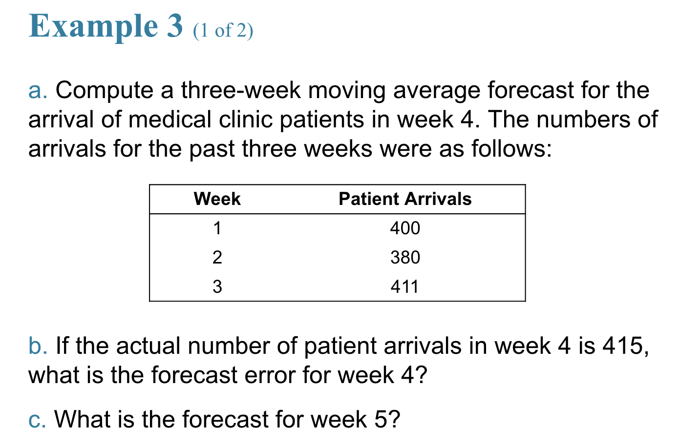
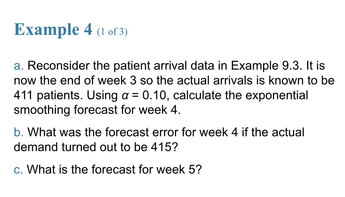
Context: A medical clinic forecasts weekly patient arrivals. Past three weeks of demand:
| Week ($t$) | Patient Arrivals ($D_t$) |
|---|---|
| 1 | 400 |
| 2 | 380 |
| 3 | 411 |
| 4 (actual) | 415 |
Example 9.3 (Simple Moving Average, $n = 3$):
- a. Compute the 3-week moving-average forecast for week 4.
- b. If actual $D_4 = 415$, what is the forecast error for week 4?
- c. What is the forecast for week 5?
Example 9.4 (Exponential Smoothing, $\alpha = 0.10$, initial forecast = 390):
- a. At end of week 3 ($D_3 = 411$), compute the exponential-smoothing forecast for week 4.
- b. Forecast error for week 4 if $D_4 = 415$.
- c. Forecast for week 5.
The forecast for the next period is the unweighted average of the most recent $n$ actual demands. Treats every period in the window equally; reacts slowly to shifts but smooths noise. Larger $n$ → smoother, slower; smaller $n$ → more responsive, noisier.
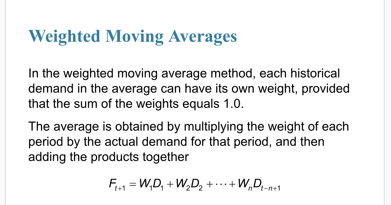
Each historical demand carries its own weight $W_i$, with $\sum W_i = 1.0$. Larger weight on recent demand → faster reaction to changes than simple MA, but still bounded by chosen weights.
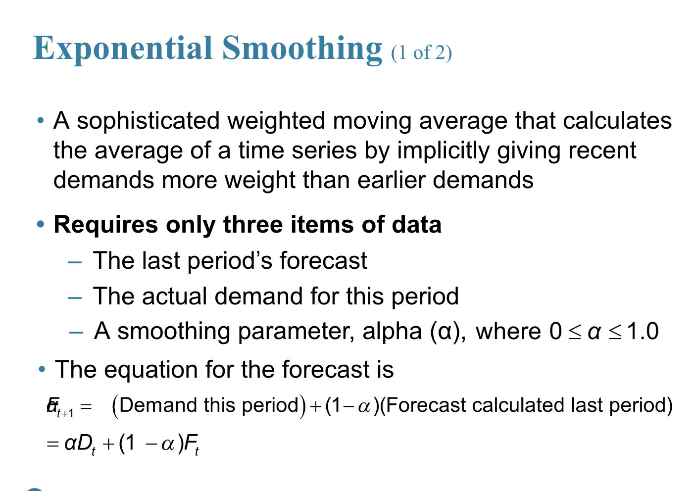
A sophisticated weighted MA that gives implicitly more weight to recent demands. Requires only 3 inputs: last period's forecast $F_t$, this period's actual $D_t$, and the smoothing parameter $\alpha \in [0, 1]$.
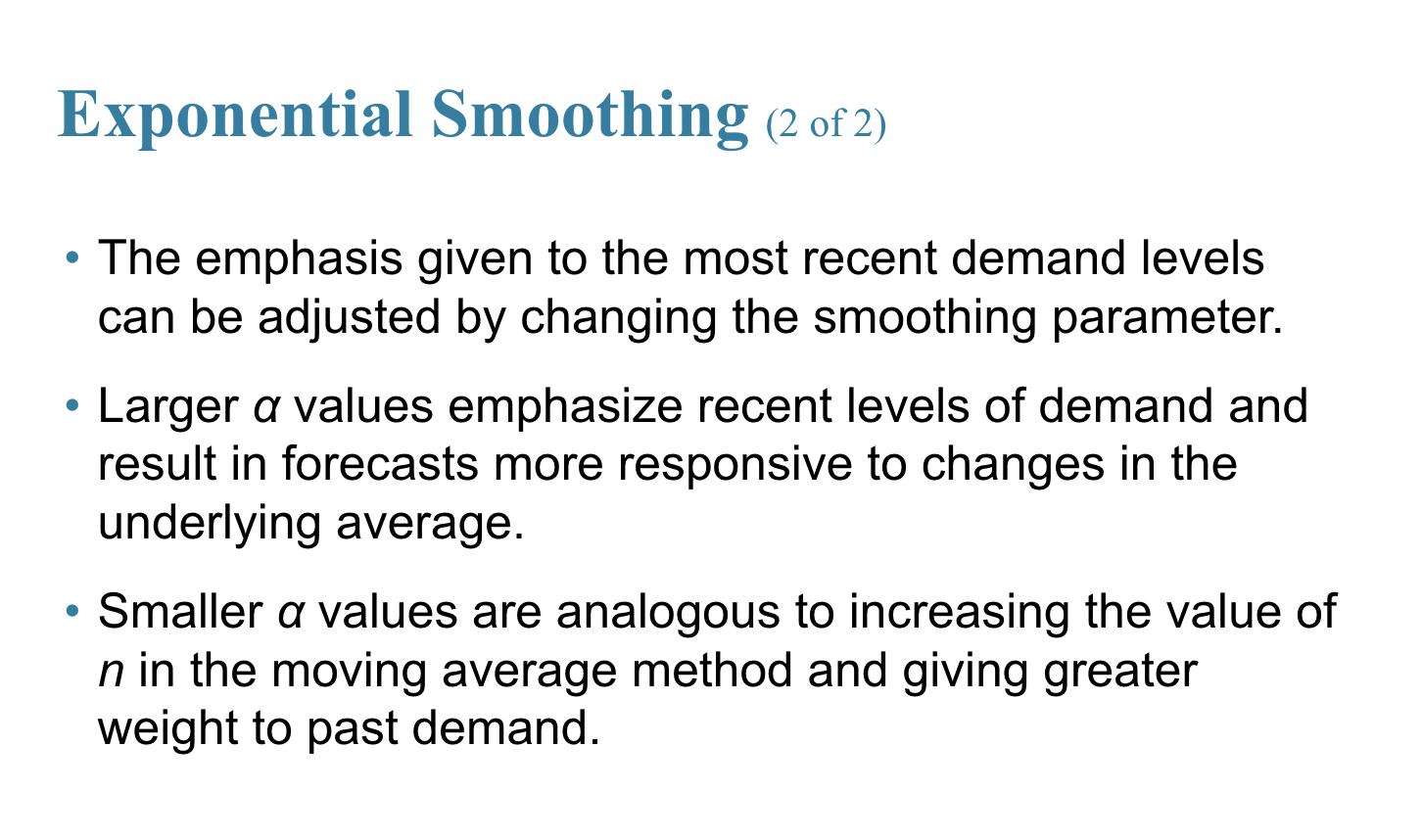
• Larger $\alpha$ → more responsive (recent emphasis).
• Smaller $\alpha$ → smoother (analogous to larger $n$ in MA).
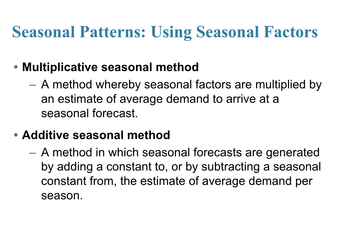
Multiplicative method: seasonal factors are multiplied by an estimate of average demand to yield the seasonal forecast.
Additive method: seasonal forecasts are produced by adding (or subtracting) a seasonal constant to/from the average-demand estimate.
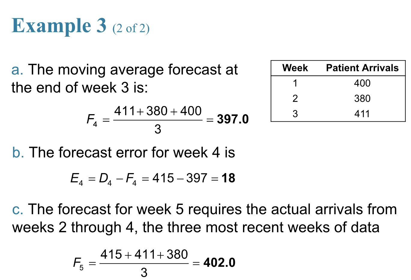
Substitute: $F_4 = \dfrac{411 + 380 + 400}{3} = \dfrac{1191}{3}$
Compute: $F_4 = \mathbf{397.0}$ patients
Substitute: $E_4 = 415 - 397$
Compute: $E_4 = \mathbf{+18}$ patients (under-forecast)
Substitute: $F_5 = \dfrac{415 + 411 + 380}{3} = \dfrac{1206}{3}$
Compute: $F_5 = \mathbf{402.0}$ patients
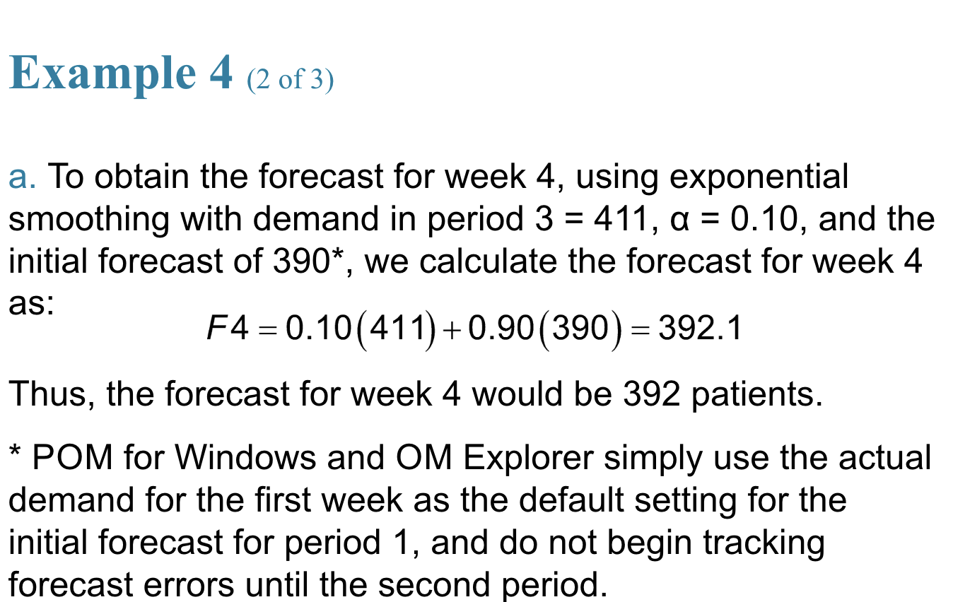
Substitute: $F_4 = 0.10(411) + 0.90(390)$
Compute: $F_4 = 41.1 + 351.0 = \mathbf{392.1} \approx 392$ patients
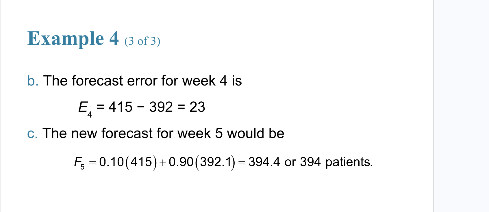
Substitute: $E_4 = 415 - 392$
Compute: $E_4 = \mathbf{+23}$ patients
Substitute: $F_5 = 0.10(415) + 0.90(392.1)$
Compute: $F_5 = 41.5 + 352.89 = \mathbf{394.4} \approx 394$ patients
| Method | $F_4$ | $E_4$ (D=415) | $F_5$ | Reaction speed |
|---|---|---|---|---|
| 3-week Moving Average | 397.0 | +18 | 402.0 | Medium — equal weight, drops oldest |
| Exponential Smoothing ($\alpha = 0.10$) | 392.1 | +23 | 394.4 | Slow — only 10% of each new observation |